


Graphs, Graph theory, Euler, and Dijkstra
As tasks become more defined, the structures of data used to define them increase in complexity. Even the smallest of projects can be broken down into groups of smaller tasks, that represent even smaller sub-tasks. Graphs are a data structure that helps us deal with large amounts of complex interactions, in a static, logical way. They are widely used in all kinds of optimization problems, including network traffic and routing, maps, game theory, and decision making. Whether we know it or not, most of us have had experiences with graphs when we interact with social media. It turns out that graphs are the perfect data structure to describe, analyze, and keep track of many objects, along with their relationships to one another. However, despite the ubiquity of graphs, they can be quite intimidating to understand. In the interest of curiosity and science, today is the day we’re going to tackle graphs, and wrestle with that uneasy feeling we get when we don’t have the slightest clue how something in front of us works.
In order to explore graphs, we’re gonna take a look at what makes a graph, cover some of the math behind it, build a simplified graph, and begin to explore a more complex social graph from Facebook data. Nodes, or vertices of a graph are like the corners of a shape, while the edges are like the sides. Edges connect with corners in all directions, giving graphs the ability to take on any shape. Any graph can be depicted with G = (V, E) , where E is the set of edges, and V is the set of vertices. Larger graphs just have more nodes, and more edges means more connectivity.
Computers find it more convenient to depict graphs as an adjacency matrix, otherwise known as a connection matrix. An adjacency matrix is made up of a square matrix that consists of only 0’s and 1’s (binary). In this binary matrix, a 1 represents a spot in the graph were an edge goes from vertex to vertex. If there is no edge running between, say vertex i and vertex j, there will be a 0 in the matrix. A good bit of graph theory can be attributed to 18th century Swiss mathematician Leonhard Euler. Euler is known as one of the most influential and prolific mathematicians of all time, with contributions in the fields of physics, number theory, and graph theory. His work on the famous Seven Bridges of Königsberg problem, where one had to decide if they could cross each bridge only once in a round-trip back to the starting point, resulted in a number of revelations concerning graph theory. Among those revelations was the discovery of the formula V-E+F=2 , having to do with the number of vertices, edges, and faces of a convex polyhedron.
Weighted, Directed, and Undirected Graphs
Weighted graphs are those that have a value associated with an edge. The weight of each edge corresponds to some cost relationship between its nodes. This cost could be distance, power, or any other relationship that relates an edge to a node. The only difference between this and an unweighted graph, is that a weighted adjacency list includes an extra field for the cost of each edge in the graph.
A directed graph is a set of objects where all the edges have a direction associated with them. You could think of most social networks as directed graphs, because direction matters when you consider the terms followers and following. Kim Kardashian certainly doesn’t follow all of her followers, rather, her 140-plus million edges are directed towards her node in a way that makes her quite influential. We’ll take a look to explore this kind of network influence a bit later when we build a graph.
Dijkstra
Edsger Dijkstra was a Dutch systems scientist, who published Dijkstra’s Shortest Path First Algorithm (SPF) in 1956. The algorithm finds the shortest paths from the source (origin) node to all other nodes. Simplified, the algorithm works under these rules:
- For each new node that is visited, choose the node with the smallest known distance/cost to visit first.
- Once at the newest node, check each of its neighboring nodes.
- For each neighboring node, calculate the cost of the neighboring nodes by summing the cost of all the edges, from the starting vertex, which lead to this node.
- If the cost to this node is less than a known (labeled) distance, this is the new shortest distance to this vertex.
- This loop continues to run through all nodes until our algorithm is done running.
Basically, this is a find and sort algorithm, where we are searching for nearby nodes, labeling them as found and measured, or found and not measured.
A Map of Manhattan
A while back, I visited some family in Manhattan. Most days I was there, I ended my trip on the Lexington Avenue line at the 125th St. station. As I walked (through the cold) from my source to wait for my train, I traversed a series of forgetful left and right turns, covering a jagged path, where the total distance was the absolute distance between turns, or Manhattan distance. Once I was underground in the subway, the train took mostly a straight line path, and that’s Euclidean distance; also known as the distance a bird flies. One weekend we decided to visit some tourist-y spots, and as we were deciding which places to visit on the map, and in which order, it looked something like this:
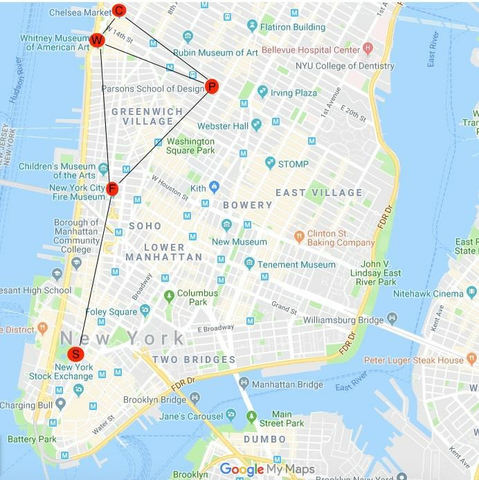
With this graph, the edges between points represent distances. If we wanted to minimize the cost from Chelsea Market © to the New York Stock Exchance (S), we could find the shortest path to S. In reality, we would want to visit all locations, but in this example we’re simply going for the absolute shortest route possible. Of course, that’s another good question: which route order signifies the shortest distance if all five destinations are desired? I may or may not leave that for you to explore on your own.
Code Exploration
All you need to have installed to explore graphs in this example is Python (preferably 3+), Matplotlib, and NetworkX. Instructions on how to properly install and get started with NetworkX can be found from their documentation. Later, we’ll download some social network data as a groundwork for analyzing much more complex graph networks. If you’d like to follow along in an interactive coding environment without having to install everything locally, the full code can be found in this IPython/Jupyter environment.
Soon, you might be surprised at how simple it is to create graph representations of many real-world objects. To start, let’s initialize a graph object, and add nodes and weighted edges to it:
import networkx as nx

import matplotlib.pyplot as plt

G = nx.Graph()

G.add_node('S')

G.add_node('F')

G.add_node('W')

G.add_node('P')

G.add_node('C')

G.add_edge('S', 'F', weight=2)

G.add_edge('F', 'W', weight=1.2)

G.add_edge('F', 'P', weight=1.5)

G.add_edge('P', 'C', weight=0.8)

G.add_edge('P', 'W', weight=1.1)

G.add_edge('W', 'C', weight=0.4)
Now, we draw the graph and label the edges:
pos = nx.spring_layout(G, scale=3)

nx.draw(G, pos,with_labels=True, font_weight='bold')

edge_labels = nx.get_edge_attributes(G,'r')

nx.draw_networkx_edge_labels(G, pos, labels = edge_labels)

plt.show()

print(nx.shortest_path(G,'C','S',weight='weight'))

print(nx.nx.shortest_path_length(G,'C','S',weight='weight'

))

all = (nx.nx.floyd_warshall(G))

print(all)
Spoiler: So I’ve already given you an idea of determining the distances from any point from the source, by using the floyd_warshall method. The returned object is a dictionary with nodes as keys, and distances as edges from the source node. You should notice that this would only solve part of our issue if we want to actually trace the path that a traveler might take if they wanted to traverse the whole route. Instead, it gives us the distance of each point from the source, not the distance between each point. Let’s keep going.
Take a look at nx.nx.spring_layout(G) . We’ve seen this before when we were setting up and drawing our graph, but we saved it in a variable, so it bears explanation. As you can see, the returned object is a dictionary of positions keyed by node. Aha! This would be the key to finding the relative positions of the nodes on a Cartesian coordinate plane. As we look back, we can see that we did in fact save these positions to the variable pos before we drew the graph. If you comment out the position step, or neglect the pos parameter in the drawing step, you’d find that the node positions would be random instead of fixed points. Effectively, just a group of connected points floating around in space, but not here; we have fixed nodes.
With the shortest_path method, we have the Dijkstra-derived algorithm tell us the final order of the shortest-first search winner, from node C to node S. You could change these parameters to come up with an alternate route if you were so inclined. If that’s not enough, we print out the length of this path, which all adds up when you do the arithmetic.
And now we play around a bit with some other functions to get more familiar with graph networks. In terms of the degree of ‘connectedness’ that each node has, you’ll use degree . That’s just going to tell us how many edges are coming out of a node. As for clustering, it is defined as:
The local clustering of each node in G is the fraction of triangles that actually exist over all possible triangles in its neighborhood. (source)
Essentially, how many nodes occupy the immediate space relative to other clusters. When you’re exploring power and influence in a network, you might look at centrality. Eigenvector_centrality gives an indication of not only how connected a node is, but how important those incoming connections are. P and W seem to be the most powerful nodes in our little network. Yet another network measure is betweenness_centrality , that tries to gauge those nodes that help form connections from distant nodes. In our example, it comes as no surprise that node F holds the throne in betweenness, effectively bridging the gap between Greenwich Village, and downtown Lower Manhattan.
Now it makes more sense why location bears so much importance in real estate, business, and other arenas. If you lack visibility within a network (city), it might be hard to turn an isolated node into a node that has high betweenness or centrality. On the other hand, you can see why office parks, malls, and strip malls can do wonders for businesses; think about those kiosks you see in airports, or vendor booths at special events.
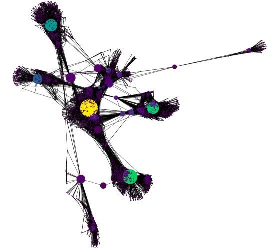
Facebook Data
Facebook means many things to many people, but one thing that cannot be argued is the vast amount of data that can be found there. If you’re looking for it, you can most certainly find it, and Stanford has cleaned up some social data for us to use. You will need to download the zip file labeled facebook_combined. When you run the code in the notebook, and properly upload your downloaded file (it gets erased on each instance) it should look something like this:

Wow – Take a deep dive into that with some of the methods we just learned!