


Table of Contents
- Overview
- Support Vector Machines (SVM) The Data
- Setup and Installation
- Exploring and Modeling the Data Takeaways
Overview
The object of this tutorial is to give you an idea of what a process might look like when a data scientist explores data with the intention of using machine learning to make predictions. Crafting a strategy to classify or regress data involves equal parts art and science, and trial and error and parameter tuning are all part of the game. For this exercise, I’ve chosen a stage ripe with data: baseball. Of course, in order to gain the most value, to be able to integrate this process into whatever projects you’re working on, you should download the data and follow along with the code, and experiment by making changes to anything you can get your hands on.
Support Vector Machines (SVM)
Before we get started, let’s first procrastinate a bit, and digest the basics of the ML algorithm we’re gonna use. Support Vector Machines are supervised machine learning algorithms that have shown success both in classification and regression since the 1960s. They have a clear method of operation that can be applied to complex problems, and for this reason, as well as their accuracy, they remain popular in modern fields, such as bioinformatics, optimization, and algorithmic trading.
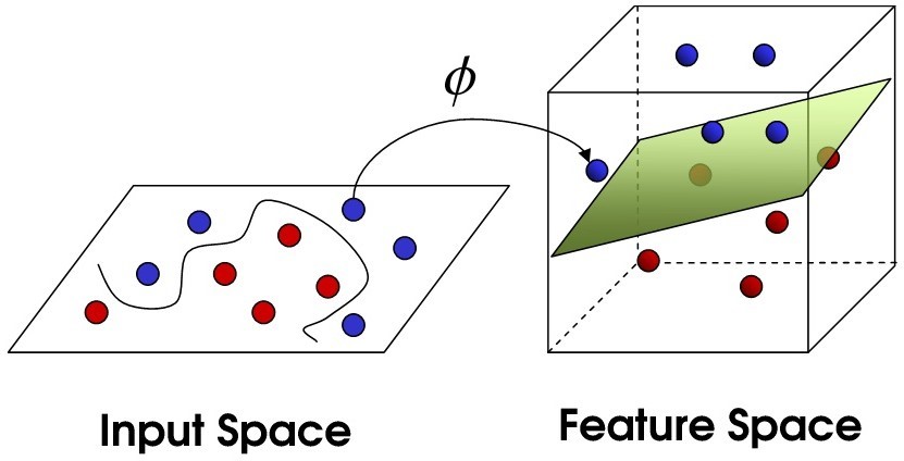
The main theme behind the workings of this machine learning algorithm, is the separation of data points in n-dimensional space, by what are called hyperplanes. Each of your features represents one n- dimension. Hyperplanes are basically separators that try to separate your classes of data into different groups, first by similarity, then by distance from one another. The object of the separation is to find the plane that maximizes the distance between classes of your data. The kicker is that during the training of your model, if there is no plane that can effectively separate the classes of data, what is known as a kernel is used to perform quite complex transformations of the data, increasing the dimensions of the data to find better hyperplanes.

SVM kernels can be linear or non-linear, so they can take complex forms that can attempt to morph to your data, often creating interesting planes of demarcation. Because they can take so many forms while finding an optimized hyperplane, tuning model parameters can lead to significantly different results. Later on, we’ll go over some solutions for how to attack this issue.
The Data
A model can’t do much without data, so let’s discuss ours, and then take a look. As it turns out, baseball can be viewed as a simple game that includes a bat, a ball, a hitter, a pitcher, and some other players; that doesn’t sound too complicated. When constructing my model, I realize that it will never replicate reality, instead, we look to simplify reality as much as possible while maximizing the accuracy of predictive outcomes. That being the case, when constructing an accurate model, the mystery is in pinning down those predictive variables which are most responsible for the outcomes. There are many ways to do this, and we will not go over them here, but you should definitely research feature selection if you want to build better models. I’ve done my own feature selection, that mostly concentrates on the pitcher-batter interaction, environment, and how well the ball will fly when hit.
The goal of each pitcher-batter interaction revolves around the fundamental action of hitting, and that involves the flight of the ball before and after a hit. Turns out that the flight of a ball is kinda complicated. After looking through some historical baseball data sources like Baseball Reference and others, and a little feature extraction, I’ve come up with some factors that I think might be important. Some of these features are taken directly from the data sources, and others are derived features, like air_dens. As I found out, the flight of the ball has to do with factors such as altitude and temperature. At higher altitudes and higher temperatures, air molecules are less densely packed, allowing balls to fly farther.
Setup and Installation
You should have Scikit Learn, Matplotlib, SciPy, NumPy, Pandas, IPython/Jupyter installed to follow along. It seems like a lot, but it’s not really much, and each of the sources provides excellent documentation to get up and running on your system. Moreover, it’ll all be up to date. We’re using Python, so surely you’ll need that.
Exploring and Modeling the Data
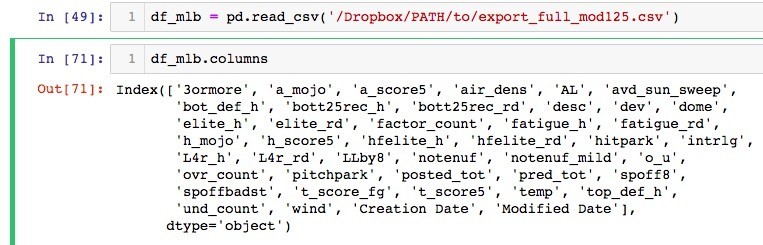
By using the Pandas command columns, we can view the columns of our dataset. Explore the size and general lay of the land with the DATAFRAME_NAME.describe() command – in this case it would be df_mlb.describe(). Looks like there are almost 600 rows of data, much of which is binary (zeros and ones), and categorical in nature. We’ve already made determinations as to whether the park is a pitcher’s park or a hitter’s park, whether the game was interleague or not, whether the game was in a dome, whether the home team had lost the last four games in a row (L4r_h), etc. Other data is continuous, like air_dens (air density), temp (temperature), etc. For this project, what’s important is how we go about predicting the total score of the game using SVM.
Preferably, open up a new Jupyter notebook, or a text editor if you don’t have Jupyter Notebook. Alternatively, Google Colaboratory may make setup a bit easier. In one cell, enter this:
cols_to_transform = ['3ormore', u'avd_sun_sweep',

'bott25rec_h', 'bott25rec_rd','elite_h',

'elite_rd','fatigue_h', 'fatigue_rd',

'hfelite_h', 'hfelite_rd', 'intrlg', 'L4r_h',

'L4r_rd', 'LLby8', 'notenuf', 'notenuf_mild',

'spoff8','spoffbadst']

df_mlb_dummies = pd.get_dummies(cols_to_transform)

clean_mlb = df_mlb.replace(['yes', 'no'], [1, 0])

clean_mlb = clean_mlb.fillna(0)
What we’ve done here is to create a list, cols_to_transform, that takes all the columns we want to make sure are categorized in a binary fashion. This will ensure that our SVM classifier can view our data as a matrix. We replace any ‘yes’ and ‘no’ categorizations with numerical 1s and 0s respectively. Let’s bring in the heavy lifters by importing the necessary modules. This is typically done at the top of our file:
from sklearn.linear_model import LinearRegression

from sklearn.ensemble import RandomForestRegressor

from sklearn.svm import SVR

from from lm = sklearn import svm

sklearn.model_selection LinearRegression() import train_test_split

from sklearn.model_selection import StratifiedShuffleSplit

from sklearn.model_selection import GridSearchCV
You should get no error messages on a successful import, but if you do, download any packages that it indicates might be missing. Next, let’s construct our classifier. Before we do so, let’s quickly browse the documentation for a list of parameters for our classifier.
sklearn.svm.SVC(C=1.0, kernel=’rbf’, degree=3,

gamma=’auto_deprecated’, coef0=0.0, shrinking=True,

probability=False, tol=0.001, cache_size=200,

class_weight=None, verbose=False, max_iter=-1,

decision_function_shape=’ovr’, random_state=None)
As you can see, there are quite a few parameters in there, dealing with kernels, gamma, degrees, etc. You could browse the docs to become more informed on those parameters – they are important. But right now, let’s not lose momentum on making baseball total score predictions.
Let’s get our classifier up and running by using a less complicated version so we can see some action:
clf = svm.SVC(gamma=0.0001, C=256,tol=0.001)

from sklearn.preprocessing import MinMaxScaler

scaling = MinMaxScaler(feature_range=(-1,1)).fit(clean_mlb[mlb_features][300:586])

X_train = scaling.transform(clean_mlb[mlb_features][300:586])
I’ve chosen to give a relatively large penalty © for error, and a gamma (kernel coefficient) of 1/1000th. This gamma parameter has to do with the sensitivity to differences in feature vectors. It depends on the degree of dimensions among other things. If gamma is too large, you may overfit your data, meaning that you will be fitting data too closely to your training set instead of fitting the data to structures that will accurately predict real-life, ground truth data. To help with support vector classification, we’ve scaled and transformed the data into an array that can be easily interpreted by the SVM. The transformed data is saved in the variable X_train.
Why did I just save rows 300 to 586? This was my way of splitting the data into training and testing sets. Sometimes, you have lots of data, and other times, with less data available, you have to use part of your data to train (X), and the rest to test dependent variables (y). There are other ways to do this, but this will work for our purposes. Now we’d like to fit the training data to our classifier:
clf.fit(clean_mlb[mlb_features][300:586],clean_mlb.t_score_fg[300:586])
Our dependent/outcome variable that we are attempting to predict, is the total score of the game, t_score_fg . Lastly, in order to see our predictions and the real outcomes of the games side-by-side, we need to construct a dataframe that displays prediction and outcome in the same table:
desc = df_mlb.ix[201:300][['desc','wind','air_dens','dev',

'spoffbadst','fatigue_rd','bott25rec_rd','bott25rec_h','t_

score5','t_score_fg]].reset_index()

desc = desc.fillna(0)

predict = pd.DataFrame(clf.predict(test_mlb[mlb_features][201:300]))

combined = pd.concat([predict,desc],axis=1)

combined.rename(columns={0: 'predict_svc'}, inplace=True) combined
Now, predict_svc gives the predictions, and t_score_fg gives the actual totals. Okay, but were these predictions any good? That depends on what you consider good. The good news is we don’t have to use our own judgement to determine the error in our model. Sklearn has a quick little method for determining the Mean Absolute Error (MAE), or the average error over the data set:
from sklearn.metrics import mean_absolute_error

y_pred = predict

y_true = test_mlb.t_score5[201:300]

mean_absolute_error(y_true, y_pred)
Using these parameters, it looks like the average total prediction is off by over 4 runs. How could we reduce this? Well, one place to start is with the parameters. While I basically arbitrarily chose the parameters, you could save time finding good parameters by having the computer do the heavy lifting. Sklearn has tools for this:
from sklearn.preprocessing import StandardScaler

from sklearn.model_selection import StratifiedKFold

from sklearn.model_selection import GridSearchCV

X, Y = clean_mlb[mlb_features][300:500],clean_mlb.t_score5[300:500]

# It is usually a good idea to scale the data for SVM trai ning.

# We are cheating a bit in this example in scaling all of the data

scaler = StandardScaler()

X = scaler.fit_transform(X)

# For an initial search, a logarithmic grid with basis

# 10 is often helpful. Using a basis of 2, a finer

# tuning can be achieved but at a much higher cost.

C_range = 2. ** np.arange(1,11)

gamma_range = 10. ** np.arange(-10, -1)

param_grid = dict(gamma=gamma_range, C=C_range)

grid = GridSearchCV(svm.SVC(), param_grid=param_grid, cv=S

tratifiedKFold())

grid.fit(X, Y)

print("The best classifier is: ", grid.best_estimator_)
This process uses grid search to find the optimal parameters to use in our SVM model. Now, if you retrain our SVM using the new, suggested clf variable, you’ll get a better model. Here are the newly suggested parameters:
clf = svm.SVC(C=2.0, cache_size=200, class_weight=None, coef0=0.0,

decision_function_shape='ovr', degree=3, gamma=1e-10, kernel='poly',

max_iter=-1, probability=False, random_state=None, shrinking=True,

tol=0.001, verbose=False)
You’ll find that it does achieve a lower MAE, but if you run the prediction again you’ll find that the same prediction is made for every game. What that means is that, given our predictive variables, our SVM model finds that you achieve the least model error by predicting a total score of 7 for every game. Well, that’s kind of a bummer, but then again, it means that our model is working pretty darn well. After all, in real baseball, a final score of around 7 or 8 could be considered the average total score. That bodes well for a nice foundation to build upon in the future.
Takeaways
Perhaps you’d like to use a Raspberry Pi or Arduino to predict the amount of water your plants need, or to determine how much food your robot food dispenser needs to give to your dogs, based on season or temperature. You could build a drone that uses a camera and an SVM to classify images into groups. The utility and useability of SVMs is high, and they run fairly fast compared to other similarly performing machine learning algorithms. We encourage you to create and experiment with this data set, and then create your own, or find some interesting publicly-available sets out there to dig into: wearable data, maps data, or whatever you can dream up.